How databases actually work

The abstraction hides too much

For the first couple of years I used databases professionally, I thought of them as smart file cabinets. You put data in, you get data out, and the database handled the details. That worked fine until I shipped a query that ran in 80ms on my local machine and 45 seconds in production against 8 million rows.

The problem wasn’t the query syntax. It was that I had no model of what the database was actually doing. Once I did, the fix was obvious. That moment is when I stopped treating databases as magic boxes.

Data lives on disk in pages

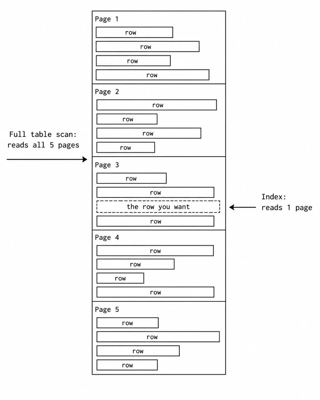
Every database stores data as pages (PostgreSQL calls them blocks, MySQL calls them pages, the idea is the same). A page is typically 8KB in PostgreSQL. It’s the smallest unit of I/O — when a database reads anything, it reads at least one full page, even if you only want one row from it.

Think about what that means for a query that needs rows scattered across a table. If you have 1 million rows spread across 80,000 pages, and your query matches 100 of them at random locations, the database might have to read 100 different pages from disk. At 10ms per random disk read (SSDs are faster but the principle holds), that’s 1 second of I/O just to return 100 rows.

This is the fundamental reason indexes exist: they let the database read far fewer pages to answer a query.

The buffer pool

Databases don’t read from disk on every query. They keep a pool of pages in memory called the buffer pool (PostgreSQL) or buffer cache (MySQL). When a query needs a page, the database checks the buffer pool first. If the page is there (a cache hit), no disk I/O happens. If it isn’t (a cache miss), the database reads it from disk and loads it into the pool.

This is why production performance often looks very different from development performance. On a fresh production database, the buffer pool is empty. Early queries are slow because every page is a cache miss. Over time, frequently accessed pages stay in memory, and the database gets faster. This “warm-up” effect catches people out constantly.

-- PostgreSQL: see how much of a table is in the buffer pool
SELECT
  relname,
  pg_size_pretty(pg_relation_size(c.oid)) AS table_size,
  pg_size_pretty(count(*) * 8192) AS cached_size,
  round(100.0 * count(*) / (pg_relation_size(c.oid) / 8192)) AS cache_pct
FROM pg_class c
JOIN pg_buffercache b ON b.relfilenode = c.relfilenode
WHERE relname = 'orders'
GROUP BY relname, c.oid;

Heap files and row storage

The main table data is stored in a heap file — rows in roughly insertion order. There’s no inherent ordering to the heap. A table with 1 million rows has those rows spread across its heap pages in whatever order they were inserted, with gaps where rows were deleted (PostgreSQL calls these “dead tuples”).

A sequential scan of a table reads every page in the heap from start to finish. It’s the simplest operation: open the file, read every page, filter rows that match the WHERE clause, return the matches. The cost scales linearly with table size.

When a table has 100 rows, a sequential scan is fine. When it has 100 million rows, a sequential scan that reads every page is almost always the wrong plan.

How storage engines differ

The storage engine is the component responsible for how data is physically stored and retrieved. PostgreSQL has one storage engine (heap). MySQL has multiple; InnoDB (the default) uses clustered indexes, which changes everything about how rows are stored.

In InnoDB, the primary key IS the physical ordering of rows on disk. The primary key B-tree contains the actual row data, not a pointer to it. This means:

• Looking up a row by primary key is fast: navigate the B-tree, you’re done.
• Every secondary index stores the primary key value (not a page pointer). Looking up by secondary index costs two B-tree lookups: one to find the primary key, one to fetch the actual row.
• Choosing a primary key carefully matters: a UUID primary key stores rows in random order, causing frequent page splits and fragmentation. An auto-increment integer stores rows in sequential order.

PostgreSQL uses heap storage with separate index structures. Every index stores a pointer (page number + offset within the page) to the actual row in the heap. This avoids the two-lookup cost for secondary indexes but means heap tuple pointers can go stale after a vacuum operation.

What a sequential scan looks like in practice

EXPLAIN ANALYZE SELECT * FROM orders WHERE customer_email = 'alice@example.com';

Seq Scan on orders  (cost=0.00..18543.00 rows=1 width=312)
                    (actual time=0.041..312.841 rows=1 loops=1)
  Filter: ((customer_email)::text = 'alice@example.com'::text)
  Rows Removed by Filter: 934999
Planning Time: 0.065 ms
Execution Time: 312.865 ms

The database read all 935,000 rows to find the one matching row. It removed 934,999 rows during filtering. The 312ms is almost entirely the cost of reading those pages.

Add an index on customer_email and the plan changes entirely. The database navigates the index, finds the matching row’s location, and fetches exactly that one page.

Index Scan using idx_orders_email on orders
  (cost=0.42..8.44 rows=1 width=312)
  (actual time=0.063..0.065 rows=1 loops=1)
  Index Cond: ((customer_email)::text = 'alice@example.com'::text)
Planning Time: 0.151 ms
Execution Time: 0.098 ms

From 312ms to 0.1ms. Same data, same query, different access path.

Why EXPLAIN ANALYZE is the first tool you reach for

Reading the query planner’s output is the most valuable database skill I have. The planner tells you exactly which operations it chose, why, and how long each one took. Without it, you’re guessing.

Key things to look for in an explain plan:

Seq Scan on a large table usually means a missing index or a predicate the planner can’t use an index for.

The rows estimate vs actual rows shows whether the planner’s statistics are accurate. A large discrepancy means statistics are stale (ANALYZE collects them) or the query pattern is unusual.

Sort + Index Scan often means the planner picked an index for filtering but then had to sort results in memory for an ORDER BY. An index that covers the sort column might help.

Nested Loop vs Hash Join vs Merge Join matters for multi-table queries. Hash joins are generally better for large datasets; nested loops are better for small ones.

The goal isn’t to make every query use an index. Sometimes a sequential scan is the right choice — if a query returns 40% of a table’s rows, reading them sequentially is faster than random index jumps. The planner usually knows this. The cases where it gets it wrong (usually due to stale statistics or unusual data distributions) are where manual analysis pays off.

Interview angles

“What’s a page in database terms?” The smallest unit of I/O. The database reads and writes data in pages (typically 8KB), not individual rows. Understanding this explains why indexes matter, why random I/O is expensive, and why buffer pool size affects performance.

“What’s the difference between a heap table and a clustered index?” A heap stores rows in insertion order with separate index structures pointing to heap locations. A clustered index (like InnoDB’s primary key B-tree) stores row data within the index itself. Clustered index lookups by primary key are one operation; heap lookups always have an extra pointer-follow step.

“Why does my query run differently in production vs development?” Usually the buffer pool. Development has a small dataset that fits in memory. Production has millions of rows and a cold cache. Other factors: different table statistics, different PostgreSQL configuration (shared_buffers, work_mem), different hardware (SSD vs spinning disk).